Kernelized Support Vector Machines

Kernelized Support Vector Machines (Kernelized SVMs) are an extension of linear support vector machines, which I covered in Chapter 2.2, that allows for more complex models. As we saw in Chapter 2.2, linear models are limiting in low-dimensional spaces because lines and hyperplanes have limited flexibility. SVMs, on the other hand, work well on both low-dimensional and high-dimensional data.

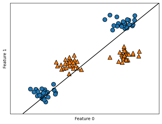
Consider the following example. Notice that a linear model can only separate points using a line, so it does a bad job on this dataset. However, by adding nonlinear features to the representation of our data (e.g. non-linear transformation feature_1 ** 2 or feature interactions feature_1 * feature_2), we can actually make linear models much more powerful. Although adding combinations of features can be computationally expensive, the kernel trick can be applied as a short cut. The mathematical reasoning behind the trick is out of the scope of the book I am studying with, but I will revisit the hardcore proofs next quarter in STAT 27700.

There are two common ways to map data into a higher-dimensional space to achieve our goal:

Using polynomial kernel: computes all possible polynomials up to a certain degree of the original features (e.g. feature_1 ** 2 * feature_2 ** 5)
Using radial basis function kernel (a.k.a. Gaussian kernel): computes all possible polynomials of all degrees with decreasing feature importance for higher degrees.

import mglearn
import matplotlib.pyplot as plt
import numpy as np
from mpl_toolkits.mplot3d import Axes3D, axes3d

from sklearn.datasets import make_blobs
X, y = make_blobs(centers=4, random_state=8) #Make 4 blobs
y = y % 2 #Seperate output into 2 classes: 0 or 1

from sklearn.svm import LinearSVC
linear_svm = LinearSVC(max_iter=5000).fit(X, y)
mglearn.plots.plot_2d_separator(linear_svm, X)
mglearn.discrete_scatter(X[:, 0], X[:, 1], y)
plt.xlabel("Feature 0")
plt.ylabel("Feature 1")

Linear Boundary

Understanding SVMs

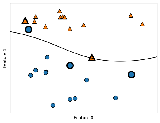
SVM works by learning how important each training data point is to represent the decision boundary between two classes. Support vectors are a subset of the training points lying on the border between two classes that matter for defining the decision boundary. Support vectors are stored in attribute support_vectors_. To make a prediction for a new point, its distance to each support vector is measured. A classification decision is then made based on the distances and the importance of each support vectors. The importance is stored in attribute dual_coef_. Also, the class of the support vectors are given by the sign of the dual coefficients. Under RBF kernel, the distance between data points is:

\[k_{RBF}(x_1, x_2) = exp(-\gamma||x_1 - x_2||^2)\]

where \(\gamma\) controls the width of the Gaussian kernel. Consider the following example to see SVM in action. Notice that it yields a smooth and nonlinear decision boundary.

from sklearn.svm import SVC

X, y = mglearn.tools.make_handcrafted_dataset()
svm = SVC(kernel='rbf', C=10, gamma=0.1).fit(X, y)
mglearn.plots.plot_2d_separator(svm, X, eps=.5)
mglearn.discrete_scatter(X[:, 0], X[:, 1], y)

sv = svm.support_vectors_ # plot support vectors
sv_labels = svm.dual_coef_.ravel() > 0 # class labels of support vectors are given by the sign of the dual coefficients
mglearn.discrete_scatter(sv[:, 0], sv[:, 1], sv_labels, s=15, markeredgewidth=3)
plt.xlabel("Feature 0")
plt.ylabel("Feature 1")

SVM Boundary

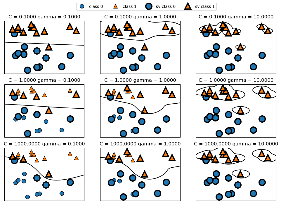
For Gaussian kernel, there are two important parameters: gamma and C. The parameter gamma controls the width of the Gaussian kernel and determines the sacle of what it means for points to be close together. A smaller gamma implies a larger radius of the kernel, which means that many points are considered to be close together. This is reflected by smoother decision boundaries (and hence a simpler model), which varies very slowly.

C is a regularization parameter that limits the importance of each point (the point’s dual_coef_). A smaller C means that each data point can only have very limited influence, and hence a simpler model.

The following shows the effects on decision boundary of these parameters. Notice that as gamma increases, data points tend to form closer and smaller groups. Further notice that as C increases, the decision boundary is made to bend to correctly classify the points.

fig, axes = plt.subplots(3, 3, figsize=(12, 8))
for ax, C in zip(axes, [-1, 0, 3]):
    for a, gamma in zip(ax, range(-1, 2)):
        mglearn.plots.plot_svm(log_C=C, log_gamma=gamma, ax=a)
axes[0, 0].legend(["class 0", "class 1", "sv class 0", "sv class 1"], ncol=4, loc=(.9, 1.2))

SVM Parameters

One drawback to SVMs is that because they are very sensitive to scaling of data, they require all features to vary on a similar scale. i.e., if there are features varying on different orders of magnitutde, kernel SVMs will do a bad job in prediction. One way to resolve this is by rescaling features so that they vary approximately on the same scale. One common rescaling method is to scale the data s.t. all features are between 0 and 1 (look into MinMaxScaler).

Other drawbacks of SVMs include:

SVMs require careful parameters setting
SVMs are hard to inspect and explain to a non-expert