Decision Trees

Decision trees are used for classification tasks. They learn a hierarcy of if/else questions (called tests) leading to a final decision. One way to visualize a decision tree is to imagine each node represents a question and each leaf the final decision, with edges of answers conecting the nodes/leaves together. If data are continuous, we ask “is feature i larger than value a” instead of “does feature i have the value a”. A prediction on a new test data point is made by traversing through the tree depending on which tests are passed and which aren’t.

To build a tree, the algorithm searches over all possible tests and finds the one that is most informative about the target variable, and thus our first test leading to two leaves is born. To increase accuracy, we repeat the process of looking for the best test in the leaves. This partitioning continues up to a specified layer or each leave contains a single class or regression value (we call such leaves pure).

Building a decision tree until all leaves are pure results in overfitting. We have two ways to prevent overfitting and control complexity:

Pre-pruning: limiting the maximum number of leaves or depth or requiring a minimum number of points in a ndoe before it can split.
Post-pruning: building the tree but collapsing nodes that contain little information.

Consider the following example that attempts to predict breast cancer. Notice our accuracy on training set is 100% since all leaves are pure, but the accuracy on testing set is worse than that on a decisioan tree with pre-pruning, demonstrating overfitting.

from sklearn.tree import DecisionTreeClassifier
from sklearn.datasets import load_breast_cancer
from sklearn.model_selection import train_test_split

cancer = load_breast_cancer() #Loads the dataset
X_train, X_test, y_train, y_test = \
    train_test_split(cancer.data, cancer.target, stratify=cancer.target, random_state=42)
tree = DecisionTreeClassifier(random_state=0).fit(X_train, y_train)
print(f"Accuracy on training set: {tree.score(X_train, y_train)}")
print(f"Accuracy on testing set: {tree.score(X_test, y_test)}")

tree = DecisionTreeClassifier(max_depth=4, random_state=0).fit(X_train, y_train)
print(f"Accuracy on training set with pre-pruning: {tree.score(X_train, y_train)}")
print(f"Accuracy on testing set with pre-pruning: {tree.score(X_test, y_test)}")

Accuracy on training set: 1.0
Accuracy on testing set: 0.9370629370629371
Accuracy on training set with pre-pruning: 0.9882629107981221
Accuracy on testing set with pre-pruning: 0.951048951048951

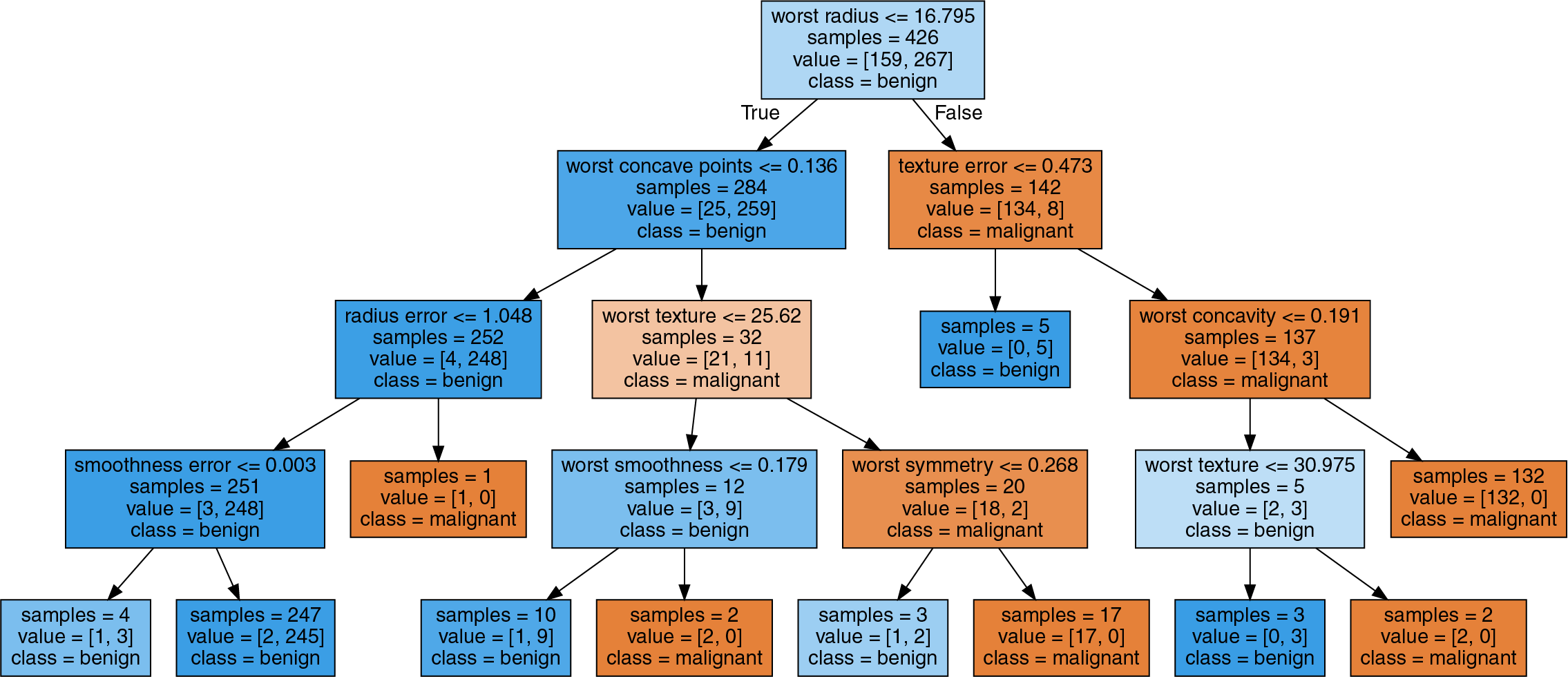
We can visualize the decision tree using export_graph from sklearn’s tree module, which writes a file in .dot format (a text file format for storing graphs). In the graph, samples gives the number of samples in that node and value provides the number of sample per class. Consider, for exmaple, we have 159 class benign and 267 class malignant in the top node, totalling to 426 samples. Also note that even though the feature “worst radius” splits the sample into 2 groups, it does not imply a monotone relationship (i.e. we do not know whether a high radius is indicative of a tumor being benign or malignant).

import graphviz
from sklearn.tree import export_graphviz

export_graphviz(tree, out_file="tree.dot", class_names=["malignant", "benign"],
    feature_names=cancer.feature_names, impurity=False, filled=True)
with open("tree.dot") as file:
    dot_graph = file.read()
graphviz.Source(dot_graph)

Decision Tree

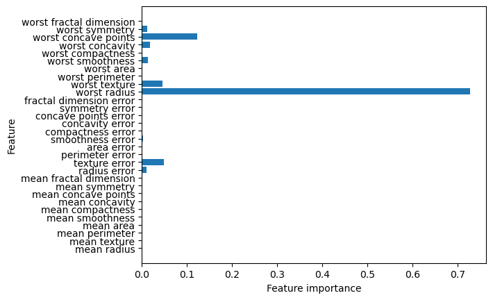
We can also check each feature’s importance in the tree-making process. This is a number between 0 and 1 where 0 means “not used at all” and 1 means “perfectly predicts the target”. Be reminded that if a feature has a low value in feature_importance_, it does not imply the feature is uninformative but rather the feature was not picked by the tree.

import matplotlib.pyplot as plt
import numpy as np

n_features = cancer.data.shape[1]
plt.barh(range(n_features), tree.feature_importances_, align='center')
plt.yticks(np.arange(n_features), cancer.feature_names)
plt.xlabel("Feature importance")
plt.ylabel("Feature")

Feature Importance

Regression Trees

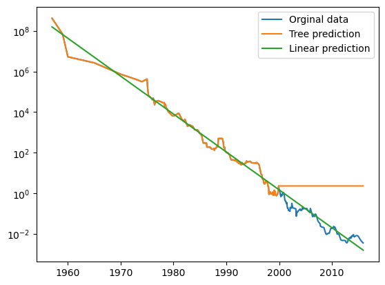
Decision tress can also be used for regression, but it cannot extrapolate (i.e. make predictions outside the range of training data).

Consider the following exmaple using a dataset of historical RAM prices per megabyte. We will make a forecast for years after 2000 using data up to that point with date as our only feature. Notice how the decesion tree makes perfect prediction on the training dsta since we did not limit complexity. It also keeps predicting the last known point once passed the data cutoff.

import pandas as pd
from sklearn.tree import DecisionTreeRegressor
from sklearn.linear_model import LinearRegression

ram_prices = pd.read_csv("Data/ram_price.csv")

data_train = ram_prices[ram_prices.date < 2000]
data_test = ram_prices[ram_prices.date >= 2000]
X_train = data_train.date[:, np.newaxis] #np.newaxis transform date array into row vector
y_train = np.log(data_train.price) #apply log to get a simpler relationship of data to target

tree = DecisionTreeRegressor().fit(X_train, y_train)
linear_reg = LinearRegression().fit(X_train, y_train)

X_all = ram_prices.date[:, np.newaxis] # predict on all data
pred_tree = tree.predict(X_all) # predict on all data
pred_lr = linear_reg.predict(X_all) # predict on all data

price_tree = np.exp(pred_tree) #undo log
price_lr = np.exp(pred_lr) #undo log

plt.semilogy(ram_prices.date, ram_prices.price, label="Orginal data")
plt.semilogy(ram_prices.date, price_tree, label="Tree prediction")
plt.semilogy(ram_prices.date, price_lr, label="Linear prediction")
plt.legend()

Regression

Decision trees have two advantages over other algorithms:

The resulting model is easily visualized and understood.
The algorithms are completely invariant to scaling of data. Therefore, no data pre-processing such as normalization or standardization is needed. Decision trees work well when features are on completely different scales or when they are a mix of discrete and continous features.