Andreas Muller & Sarah Guido - Introduction to Machine Learning with Python - Chapter 2.2

Supervised Learning with Linear Models

Linear models make prediction using a linear function of the input features. The model looks as follows:

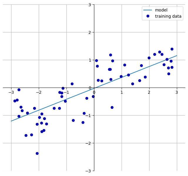
\[\hat{y} = \beta + w_0x_0 + w_1x_1 + ... + x_{p-1}x_{p-1}\]

where \(x_i\) denotes the i-th featue of a single data point, \(w_i\) and \(\beta\) are parameters of the model, and \(\hat{y}\) is the prediction made. For a model with only 1 feature, the equation is reduced into a simple equation of line. To illustrate how the model works, we will use the same datasets as before and plot a graph with linear model in effect. Notice the slope of line is ~0.4, which is what w[0] is, and the y-intercept is ~0, which is what b is.

import matplotlib.pyplot as plt
import numpy as np
import mglearn #Package that comes with the textbook
X, y = mglearn.datasets.make_forge() #Import data, x is input, y is output
A, b = mglearn.datasets.make_wave(n_samples=40)

mglearn.plots.plot_linear_regression_wave()

Linear Regression

Linear regression, a.k.a. ordinary least squares (OLS), finds coefficients w and b that minimize the mean squared error, \(\frac{1}{n}\sum_{i=1}^{n}(Y_i-\hat{Y_i})^2\), between predictions and the actual targets, y. Linear regression models has no parameters, so we cannot adjust model complexity. Coincidentally, I just learned the hardcore maths behind the model 2 hours before I was writing this note, it amazes me how much is abstrated away from us when using sklearn. When scoring the accuracy of the model, \(R^2\) is used. With higher-dimensional datasets, linear models are more powerful but are also more likely to overfit.

from sklearn.linear_model import LinearRegression
from sklearn.model_selection import train_test_split
A_train, A_test, b_train, b_test = train_test_split(A, b, random_state=0)

lr = LinearRegression() #initiate linear regression model
lr.fit(A_train, b_train) #fit data into model
print("w:", lr.coef_, "and b:", lr.intercept_) #coeffient lst and y-intercept
#name_ indicates something derived from training data
print("Training score:", lr.score(A_train, b_train))
print("Test score", lr.score(A_test, b_test))

w: [0.52424272] and b: -0.09394309015377247
Training score: 0.6883322630458479
Test score 0.626150295776388

Ridge Regression

Ridge regression similar to OLS, but introduces one regularization to avoid overfitting: the coefficients, w, are chosen to preidct well on the training data while minimizing their magnitudes. We call this the L2 regularization. In this way, each feature has only a little effect on the outcome.

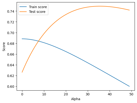
Note that the accuracy on the training set decreases, but that on the test set increases. This is consistent with out expectation that ridge regression lowers the risk of overfitting and improves generalization. Ridge regression is particularly more powerful than OLS when we have fewer data points, because regularization becomes less important as the number of data points increases.

from sklearn.linear_model import Ridge
rr = Ridge().fit(A_train, b_train) #Method chaining, initialize then fit data
print("w:", rr.coef_, "and b:", rr.intercept_)
print("Training score, default alpha:", rr.score(A_train, b_train))
print("Test score, default alpha", rr.score(A_test, b_test))

w: [0.51833613] and b: -0.09493454237048432
Training score, default alpha: 0.6882448839910054
Test score, default alpha 0.6355755075905882

Further, the extent to which we want to limit the magnitude of coefficients can be controlled by setting parameter alpha (default is 1). The higher the alpha, the more coefficients are to move towards 0, which may further improve generalization.

alphas = np.arange(0, 50, 1)
train_score, test_score = [], []
for a in alphas:
    rr = Ridge(alpha=a).fit(A_train, b_train)
    train_score.append(rr.score(A_train, b_train))
    test_score.append(rr.score(A_test, b_test))

plt.plot(alphas, train_score)
plt.plot(alphas, test_score)
plt.legend(["Train score", "Test score"])
plt.xlabel("Alpha")
plt.ylabel("Score")

Lasso

Lasso is another kind of linear regression that also restricts coefficients to be close to 0 under L1 regularization, under which some coefficients are exactly 0 (influence of some features are ignored). To demonstrate automatic feature selection, we import another dataset that has 105 features. Note that we default alpha, the model underfits, hence we will decrease alpha. At the same time, as alpha decreases, we reduce the strength of regulation, and the computation may not converge without increasing the maximum number of iterations.

In practice, ridge regression is preferred over lasso unless we specifically want automatic feature selection. In general, we prefer L2 than L1 unless we specifically want feature elimination. ElasticNet is another linear regression model that offers both L1 and L2.

%%capture
A, b = mglearn.datasets.load_extended_boston()
A_train, A_test, b_train, b_test = train_test_split(A, b, random_state=0)

from sklearn.linear_model import Lasso
lasso = Lasso(alpha=0.01, max_iter=100000).fit(A_train, b_train)
print("Training score, default alpha:", lasso.score(A_train, b_train))
print("Test score, default alpha", lasso.score(A_test, b_test))
print("Features used:", np.sum(lasso.coef_ != 0), "out of 105")

Training score, default alpha: 0.8962226511086497
Test score, default alpha 0.7656571174549983
Features used: 33 out of 105

Linear Models for Classification

Linear models can also be used in classification problems using the following formula:

\[\hat{y} = \beta + w_0x_0 + w_1x_1 + ... + x_{p-1}x_{p-1} > 0\]

If the prediction is smaller than 0, we classify it as -1, otherwise we classify it as +1. Notice that the decision boundary is a linear function of the input (i.e., the model separates two classes using the line given by the equation).

Logistic regression and Linear support vector machines are two commonly used linear classification algorithm. They both apply L2 regularization (w are minimized) by default, which is controlled by parameter C. Similar to alpha in Ridge regression but in the opposite direction, a lower value of C tells the model to put more strength onto minimizing w and hence a simpler model. One way to think about this is that higher C imples higher democracy: using low values of C will cause the algorithms to try to adjust to the “majority” of data points, while using a higher value of C stresses the importance that each individual data point be classified correctly. One can also change the regularization to L1 with argument penalty="l1".

Note again that linear models for classficication are restrictive in low-dimensional spaces because it may be impossible to seperate two classes perfectly using a singly straight line, but as dimension increases, so does the power of the models and its guard against overfitting.

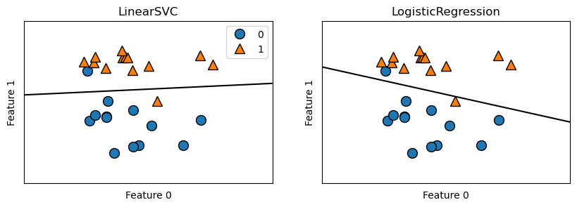
Figure below shows the decision boundary under the two models, with data points lying on the upper region classified as class 1, and data points lying on the lower region classified as class 2. The shape and color of data points show their actual class.

from sklearn.linear_model import LogisticRegression
from sklearn.svm import LinearSVC

fig, axes = plt.subplots(1, 2, figsize=(10,3))
for model, axis in zip([LinearSVC(max_iter=5000), LogisticRegression()], axes):
    classification = model.fit(X, y)
    mglearn.plots.plot_2d_separator(classification, X, ax=axis)
    mglearn.discrete_scatter(X[:, 0], X[:, 1], y, ax=axis)
    axis.set_title(f"{classification.__class__.__name__}")
    axis.set_xlabel("Feature 0")
    axis.set_ylabel("Feature 1")
axes[0].legend()

Linear Models for Multiclass Classification

One technique to extend a binary classification algorithm to a multiclass classification algorithm is the one-vs-rest approach. In it, for each class of the n classes, a binary model is learned and tries to separate that class from the all other classes. This way, we will obtain n many binary models. To make a prediction, all models are applied on the same point, and the model (i.e. the forumula) that yields the highest \(\hat{y}\) wins. Note that having one binary classifier per class implies having a vector of coefficients (w) and an intercept (b).

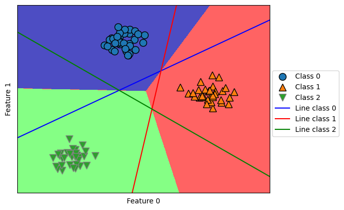
The following demonstrates the approach. Note that after fitting the model, coefficient is a 3-by-2 matrix since we have 3 classes and 2 features, and intercept is a 3-by-1 vector since we have 3 classes. In the figure, notice that the points of a class are separated from the rest of the points by their respective decision boundry line. Moreover, if test points are located at the center triangle, they are classified into the class of the closest line.

from sklearn.datasets import make_blobs
X, y = make_blobs(random_state=42)

linear_svm = LinearSVC().fit(X, y)
mglearn.discrete_scatter(X[:, 0], X[:, 1], y)
mglearn.plots.plot_2d_classification(linear_svm, X, fill=True, alpha=.7)
line = np.linspace(-15, 15)
for coef, intercept, color in zip(linear_svm.coef_, linear_svm.intercept_, \
    ['b', 'r', 'g']):
    plt.plot(line, -(line * coef[0] + intercept) / coef[1], c=color)
plt.legend(['Class 0', 'Class 1', 'Class 2', 'Line class 0', 'Line class 1', \
    'Line class 2'], loc=(1.01, 0.3))
plt.xlabel("Feature 0")
plt.ylabel("Feature 1")

A few remarks after this long chapter:

1. One may consider using argument solver="sag" in logistic regression or ridge when working with large sample set and want faster computation.
2. SGDClassifier and “SGDRegressor* implement more scalable versions of the linear models mentioned above.
3. Linear models often perform well when the number of features is large compared to the number of samples.