Andreas Muller & Sarah Guido - Introduction to Machine Learning with Python - Chapter 2.1
Supervised Learning with k-NN Algorithm
Supervised Learning is used when we want to predict a certain outcome from a given input, and we already have examples of input-output pairs. The goal here is to make accurate predictions for new data as inputs.
There are two types of supervised ML problems:
- Classification: the goal is to predict a class label. Binary classification is the case of distringuishing between exactly two classes (a Y/N question).
- Regression: the goal is to predict a continuous number.
We say a model is able to generalize from the training set to the test set if accurate predictions are made on new data. We always want to find the simplest model to avoid overfitting, but not so simple that it underfits. Large datasets with varying data and features (high-dimensional datasets) allow building more complex models.
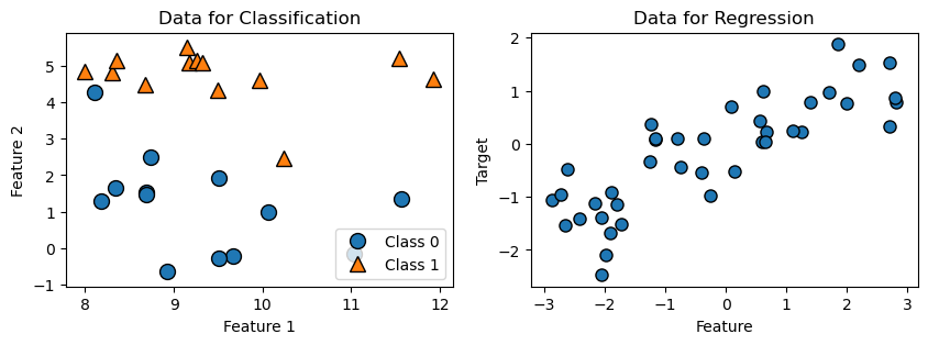
In the following, 2 datasets are prepared to illustrate the simplest machine learning model, the k-Nearest Neighbor Model:
- The first dataset has 26 data points and 2 features. Each data point is a dot, and the appearance of the dot indicates its class. This dataset is used for two-class classification demonstration.
- The second dataset has 40 data points and 1 feature. This dataset is used for regression demonstration.
import matplotlib.pyplot as plt
import mglearn #Package that comes with the textbook
X, y = mglearn.datasets.make_forge() #Import data, x is input, y is output
A, b = mglearn.datasets.make_wave(n_samples=40)

fig, axes = plt.subplots(1, 2, figsize=(10, 3))
mglearn.discrete_scatter(X[:, 0], X[:, 1], y, ax=axes[0]) #.scatter adaptation
axes[0].set_title("Data for Classification")
axes[0].set_xlabel("Feature 1")
axes[0].set_ylabel("Feature 2")
axes[0].legend(["Class 0", "Class 1"], loc=4)
mglearn.discrete_scatter(A, b, ax=axes[1], s=8)
axes[1].set_title("Data for Regression")
axes[1].set_xlabel("Feature")
axes[1].set_ylabel("Target")
Text(0, 0.5, 'Target')
Two-class Classification with K-Nearest Neighbours Alogorithm
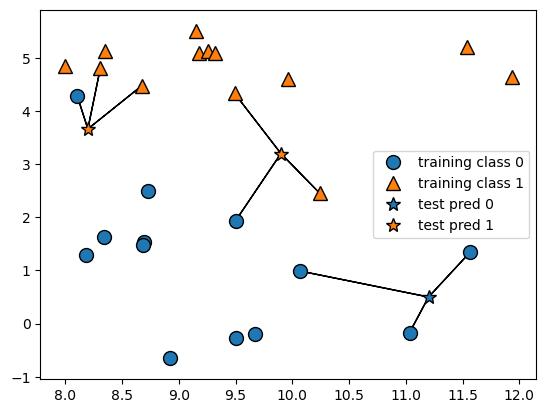
The k-Nearest Neighbors (k-NN) algorithm finds k-many of the closest data points in the training dataset and classify them as one category. Building the model consists only of storing the training dataset. We feed the model 1 data point for prediction, then k-NN algoritgm considers k many of its nearest neighbors’ classes, and classifies our testing data as the class that is the most frequent.
#Stars: points we want to make prediction for; circles :training points
mglearn.plots.plot_knn_classification(n_neighbors=3)
#Split dataset into training and testing data
from sklearn.model_selection import train_test_split
X_train, X_test, y_train, y_test = train_test_split(X, y, random_state=0)

from sklearn.neighbors import KNeighborsClassifier
clf = KNeighborsClassifier(n_neighbors=3) #initiate model class
clf.fit(X_train, y_train) #fit data into model, parameters: (features, output)
print("Predictions:", clf.predict(X_test)) #make prediction w/ test feature data
print("Accuracy:", clf.score(X_test, y_test)) #Percentage of correct prediction
Predictions: [1 0 1 0 1 0 0]
Accuracy: 0.8571428571428571
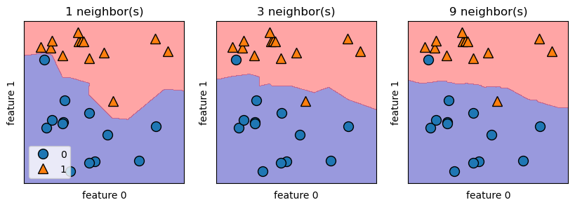
We can illustrate the prediction for all possible points on the xy-place using decision boundary. For k-NN algorithm, a smoother boundary implies a lower model complexity. In the figure below, if data point lies on the red area, then it belongs to group 1, otherwise it belongs to group 0. Notice that as k increases, the decision boundary follows the training data less closely and becomes smoother. Hence, large enough k will lead to underfitting.
fig, axes = plt.subplots(1, 3, figsize=(10, 3))
for n_neighbors, ax in zip([1, 3, 9], axes):
    clf = KNeighborsClassifier(n_neighbors=n_neighbors).fit(X, y)
    mglearn.plots.plot_2d_separator(clf, X, fill=True, eps=0.5, ax=ax, alpha=.4)
    mglearn.discrete_scatter(X[:, 0], X[:, 1], y, ax=ax)
    ax.set_title("{} neighbor(s)".format(n_neighbors))
    ax.set_xlabel("feature 0")
    ax.set_ylabel("feature 1")
axes[0].legend(loc=3)
<matplotlib.legend.Legend at 0x2433188bf70>
Regression with K-Nearest Neighbours Alogorithm
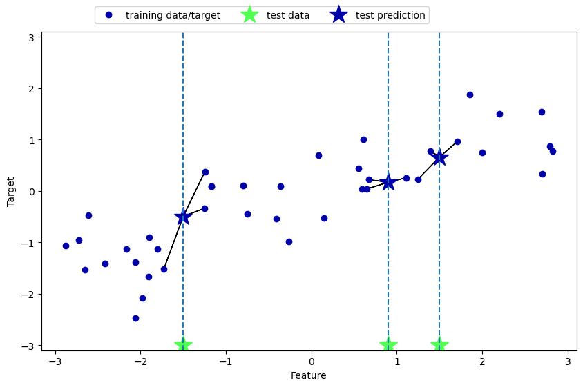
The application of k-NN algorithm on continuous data is also straightforward: we feed the model 1 data point for prediction, it then records the target value of its k nearest neighbors, and returns the mean as the predicted value. The accuracy score returned here is the R^2 score that measures the goodness of fit (the smaller the better).
mglearn.plots.plot_knn_regression(n_neighbors=3)
from sklearn.neighbors import KNeighborsRegressor
A_train, A_test, b_train, b_test = train_test_split(A, b, random_state=0)
reg = KNeighborsRegressor(n_neighbors=3) #initiate the regression model
reg.fit(A_train, b_train)
print("Predictions:", reg.predict(A_test))
print("Accuracy:", reg.score(A_test, b_test)) #b_test checks A_test predictions
Predictions: [-0.05396539  0.35686046  1.13671923 -1.89415682 -1.13881398 -1.63113382
  0.35686046  0.91241374 -0.44680446 -1.13881398]
Accuracy: 0.8344172446249605
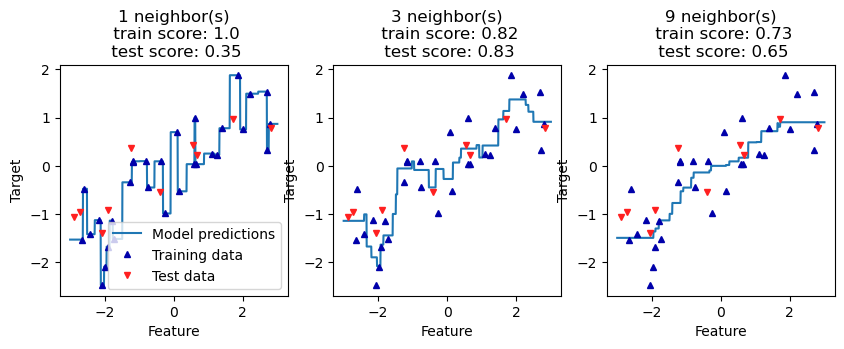
Note that again as k increases the prediction curve gets smoother, but also increases the risk of underfitting.
fig, axes = plt.subplots(1, 3, figsize=(10, 3))
# create 1,000 data points, evenly spaced between -3 and 3
line = np.linspace(-3, 3, 1000).reshape(-1, 1)
for k, ax in zip([1, 3, 9], axes):
    # make predictions using 1, 3, or 9 neighbors
    reg = KNeighborsRegressor(n_neighbors=k)
    reg.fit(A_train, b_train)
    train_s = round(reg.score(A_train, b_train), 2)
    test_s = round(reg.score(A_test, b_test), 2)
    ax.plot(line, reg.predict(line))
    ax.plot(A_train, b_train, '^', c=mglearn.cm2(0), markersize=5)
    ax.plot(A_test, b_test, 'v', c=mglearn.cm2(1), markersize=5)
    ax.set_title(
        f"{k} neighbor(s)\n train score: {train_s}\n test score: {test_s}")
    ax.set_xlabel("Feature")
    ax.set_ylabel("Target")
axes[0].legend(["Model predictions", "Training data", "Test data"])
<matplotlib.legend.Legend at 0x2432fd29a20>
There are two important parameters to K-NN algorithm:
- Number of neighbors: 3 - 5 neighbors work well
- How we measure distance: Euclidean distance is often used
The strength of k-NN is its ease to understand and reasonable performance without complicated adjustments. However, applying k-NN models on large datasets can be slow. It also yields poor performance if the dataset has many features or is sparse (most features are 0 most of the time).